Academia.edu uses cookies to personalize content, tailor ads and improve the user experience. By using our site, you agree to our collection of information through the use of cookies. To learn more, view our Privacy Policy.
Doing the right things–trivalence in deontic action logic
Last updated Robert Trypuz
 Piotr Kulicki
…
106 pages
Sign up for access to the world's latest research
Abstract
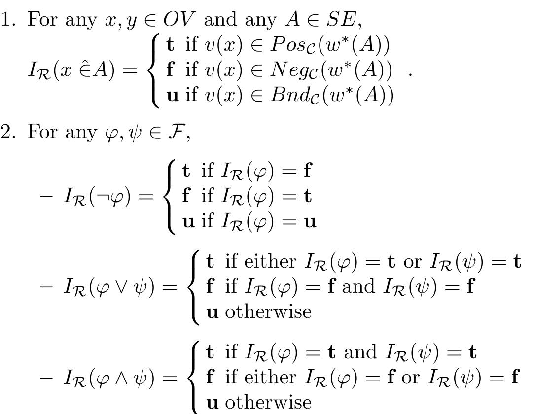
Abstract. Trivalence is quite natural for deontic action logic, where actions are treated as good, neutral or bad. We present the ideas of trivalent deontic logic after J. Kalinowski and its realisation in a 3-valued logic of M. Fisher and two systems designed by the authors of the paper: a 4-valued logic inspired by N. Belnap's logic of truth and information and a 3-valued logic based on nondeterministic matrices. Moreover, we combine Kalinowski's idea of trivalence with deontic action logic based on boolean algebra.
![This choice concerning the third truth value highlights the distinction be- tween paracomplete and paraconsistent interpretations of trivalent logic. In light of the bivalent interpretation, four new truth values can therefore be defined (see [2]). Let ({t, f,n, b}, <) be a lattice such that:](https://figures.academia-assets.com/30815618/figure_001.jpg)
![resents human knowledge. /Injerential adequacy Measures whether the compu- tations behave similarly to human reasoning. It is straightforward to see that classical two-valued logic cannot model the suppression task adequately. At least a non-monotonic operator is needed. Stenning and van Lambalgen [1] suggest that human reasoning is modeled by, firstly, reasoning towards an appropriate representation or logical form (conceptual adequacy) and, secondly, reasoning with respect to this representation (inferential adequacy). As appropriate repre- sentation to model the suppression task, Stenning and van Lambalgen propose ogic programs under completion semantics based on the three-valued logic used by Fitting [3], which itself is based on the three-valued Kleene [4] logic. Un- ortunately, some technical claims made by Stenning and van Lambalgen [1] are wrong. Hélldobler and Kencana Ramli [5] have shown that the three-valued ogic proposed by Fitting is inadequate for the suppression task. Somewhat sur- prisingly, the suppression task can be adequately modeled if the three-valued Lukasiewicz [6] logic is used. The computational logic approach in [5,7] models the suppression task as logic programs together with their weak completion. They show that the conclusions](https://figures.academia-assets.com/30815618/table_001.jpg)
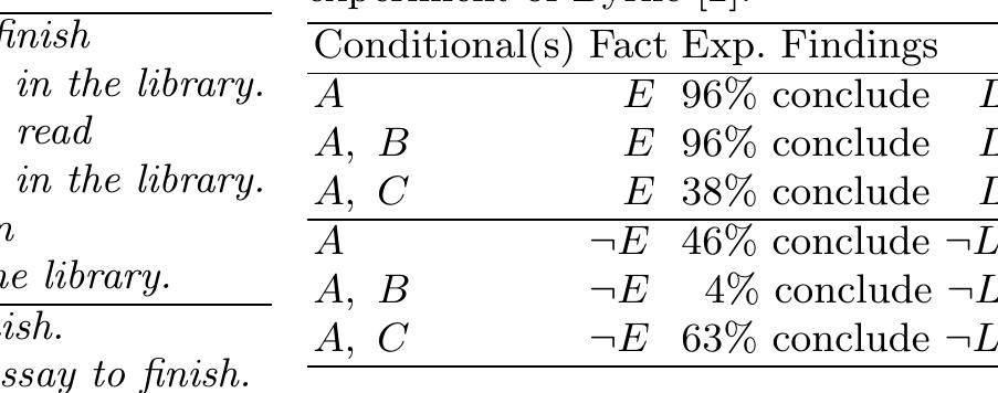
![Table 4. Representational Form of the Suppression Task 3.3. Reasoning Towards an Appropriate Logical Form Stenning and van Lambalgen [1] have argued that the first step in modeling hu- man reasoning is reasoning towards an appropriate logical form. In particular, ™, ™, but rat Table 4 shows the representational pression task as modeled by Stenning and van Lambalgen.! The last column of Table 4 shows the findings of Byrne The predicates ab;, abz and abs represent different kinds of abnormality. For in- stance, Pape and Pacer contain two i. Both programs differ in the way clause is an alternative to the first c ond clause is an additional to the first clause. The difference is represented by the additional clause in P4cg where ab; is true when The library does not stay open and abs is true when She does not have an essay to finish. We assume that Stenning and van Lambalgen adequately model this part of the suppression task and adopt this reasoning step. they argue that conditionals shall not be encoded by implications straight away her by licenses for implications. For example, the conditional A in Ta- ble 1 should be encoded by the clause | + eA 7ab;, where ab; is an abnormality predicate which expresses that something abnormal is known. In other words, | holds if e is true and nothing abnormal is known. orm of the first six examples of the sup- 2]. clauses which yield to the same conclusion hat for Paper, the premise of the second ause and in P4cg the premise of the sec- Stenning and van Lambalgen [1] have argued that the first step in modeling hu- man reasoning is reasoning towards an appropriate logical form. In particular, they argue that conditionals shall not be encoded by implications straight away but rather by licenses for implications. For example, the conditional A in Ta- ble 1 should be encoded by the clause | + eA -ab,, where ab, is an abnormality predicate which expresses that something abnormal is known. In other words, | holds if e is true and nothing abnormal is known. Thalele A dhe thn samrecontoadiiwesd | Lae: nh the Beat offer qeenernesdec: nf Phan: oes.](https://figures.academia-assets.com/30815618/table_003.jpg)
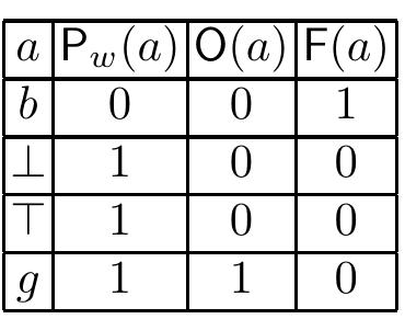
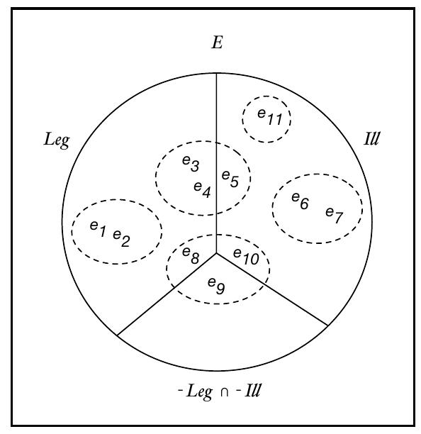
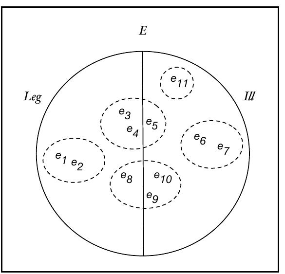
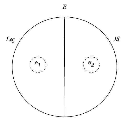
![Additionally we accept that the interpretation of every atom is a singleton: set of possible outcomes (events), Leg and [1] are subsets of F and should be un- derstood as sets of legal and illegal outcomes respectively. The basic assumption is that there is no outcome which is legal and illegal: where 6 is an atom of Act. A basic intuition is such that an atomic action corre- sponding to (a set with) one event/outcome is indeterministic. It is important to note two things in this place. The first one is that Z(d) is a subset of either Leg. or Ill or —LegM —Ill and the second one is that in every situation an agent’s action has only one outcome, which means in practice that what agents really do is to carry out atomic actions.](https://figures.academia-assets.com/30815618/table_008.jpg)
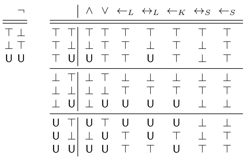
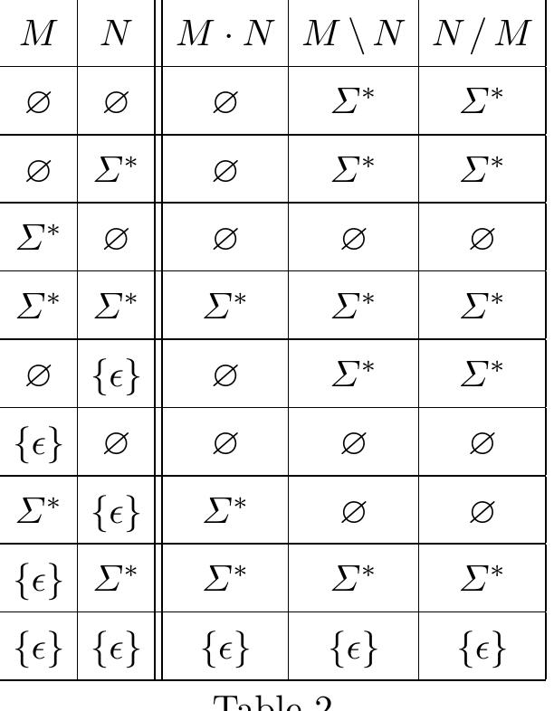
![The first four rows here just represent truth tables for classical conjunction and implication; the other rows extend these operations to their three-valued versions: = is the implication of Sobocitiski’s [9] logic RM3 (a Gentzen-style calculus for it can be found in [1]), & is the contenability (fusion) operation. We shall say that a value x € T is “true” if x = 1 or x = 1, and “false” if r = 0. We also introduce an ordering on T:0<1< 1.](https://figures.academia-assets.com/30815618/table_010.jpg)
![In this section we consider L-models with a special constant 0, interpreted as 2. The set of types here is denoted by Tp. We introduce a new set T = {0,1, 7}, and two new operations &,=>: T x T — T, defined as follows (this is the implication-conjunction fragment of the strong Kleene [3, § 64] 3-valued logic): Lhe trivalent interpretation T 1s denned as in the previous section; T(Q) = U. Now we introduce a hybrid logic Lo: we say that Lo — G (G € Tpg) if either 7(G) = 1 for any trivalent interpretation 7, or for any trivalent interpretation 7 we have 7(G) € {1,4}, and L - > G (in L-derivations 0 is considered an ordinary primitive type). We say that Lo | F\...Fim — G iff Lo - = (F,-...+ Fin) \G.](https://figures.academia-assets.com/30815618/table_012.jpg)
Related papers
Journal of Applied Logic, 2009
We introduce a deontic action logic and its axiomatization. This logic has some useful properties (soundness, completeness, compactness and decidability), extending the properties usually associated with such logics. Though the propositional version of the logic is quite expressive, we augment it with temporal operators, and we outline an axiomatic system for this more expressive framework. An important characteristic of this deontic action logic is that we use boolean combinators on actions, and, because of finiteness restrictions, the generated boolean algebra is atomic, which is a crucial point in proving the completeness of the axiomatic system. As our main goal is to use this logic for reasoning about faulttolerant systems, we provide a complete example of a simple application, with an attempt at formalization of some concepts usually associated with fault-tolerance.
2026
We investigate here the connectives of the three-valued logical systems of Lukasiewicz, Kleene and Heyting using matrix operators and vector truth values. Several novel results follow from this formalism. The modalities possibility and necessity are represented by monadic matrices. These modalities, and other monadic connectives, are represented by idempotent matrices and these idempotent matrices have square roots which, in turn, are logical connectives. Lukasiewicz's implication allows, from simple matrix operations, to generate a Polish variety of conjunction and disjunction. These connectives allow the creation of a three-valued and modal variant of implication based on the new Polish conjunction. Heyting's intuitionistic logic has two possible definitions of negation and shows, from its matrix formulation, its essentially modal nature. In fact, one negation corresponds to non-possibility and the double negation is identical to the possibility matrix; the other negation corresponds to non-necessity and the double negation is the matrix of necessity. Furthermore, Heyting's logical matrices verify the axioms established by Heyting's intuitionistic logic. The matrix analysis of De Morgan's pseudo-laws arising from Heyting's formal system converts them into identities between matrix operators.
The Logica Yearbook 2011
The aim of the paper is to point out the modelling choices that lead to different systems of deontic action logic. A kind of a roadmap is presented. On the one hand it can help the reader to find the deontic logic appropriate for an intended application relying on the information considering the way in which a deontic logic represents actions and how it characterises deontic properties in relation to (the representation of) actions. On the other hand it is a guideline how to build a deontic action logic which satisfies the desired properties.
Deontic Logic in Computer Science 2012, 2012
"We start our investigations from the deontic action model defined in multi-situation settings. Then we discuss the validity of formulas constructed in a language with a finite number of basic actions, parallel and sequential compositions of actions, a free choice operator and the standard deontic operators of obligation, strong permission and prohibition. The main achievements of the paper are definitions of metalogical counterparts of deontic operators and interpretation function of actions taking into account their terminating and non-terminating executions."
“The logic of best action from a deontic perspective” and “Obligation, free choice and the logic of weakest permission” argued that, in games, obligations and permissions should be viewed, respectively, as giving necessary and sufficient conditions for rationality. This gives rise to a specific deontic logic where, for instance, O and P are not dual notions and P becomes a “free choice” permission operator. Similar deontic logics have been proposed in the literature, as early as van Benthem’s Minimal deontic logics, and more recently in “On deontic action logics based on boolean algebra”. In this paper we study the relation between these deontic logics for rational agency in games. We compare their deductive power, provide translation results, and emphasize the different views they take on what players ought to, or may do.
Studia Logica
This paper tackles the problem of inference in normative systems where norms concerning actions and states of affairs appear together. A deontic logic of actions and states is proposed as a solution. It is made up of two independent deontic logics, namely a deontic logic of action and a deontic logic of states, interlinked by bridging definitions. It is shown at a language and a model level how an agent should look for norms to follow in a concrete situation. It is pointed out that such specific norms are obtained by finding the most specific obligation and the most general prohibition. They are to be derived from all norms applicable to the situation by using the principles of the logic presented in this paper.
In their novel “The Difference Engine”, William Gibson and Bruce Sterling accomplish the feat of imagining that computer science developed from the investigations of Charles Babbage, Ada Lovelace, and from the formalisms that followed those achievements. All of this is implicit in the Babbage text that the authors place at the end of the book (“The Language of Signs” inspired by Lord Charles Babbage, “Passages from the Life of a Philosopher”, 1864.) But the period that inspired Gibson and Sterling's fiction, was extraordinarily influential in multiple domains of science. In mathematics, it led to the intense development of operator theory, and it was within this framework that George Boole produced his revolutionary algebraic theory of logic between 1847 and 1854. Shortly thereafter, Cayley created the theory of matrices and Peirce had the vision of using this theory to deal with some aspects of logic. However, the use of matrix algebra in logic came to a halt. The emergence of Frege's formalisms and that of Whitehead and Russell transformed logic into a virtual instrument for investigating the foundations of mathematics, and the enormous achievements of this line of research, which perhaps culminates in the enormous contributions of Gödel and Turing, need not be emphasized. But since the beginning of the 21st century, vigorous developments in quantum computing research have taken up matrix algebra as one of its basic techniques. The research reported in this monograph is based on a matrix formalism of logic originating in neural models developed in the late 1980s. Matrix algebra provides a surprisingly simple procedure for addressing relevant topics in basic logic and, in particular, in many-valued logics. Here we investigate the relationships among three relevant systems of three-valued logics, postulated in different contexts by their authors. These are: Lukasiewicz's logic, which combines philosophical roots with the technical search for mathematical formalisms for modalities; Kleene's logic, inspired by decidability problems in formal systems; and Heyting's logic, which succeeded in defining a three-valued logic that encompasses the fundamental properties of intuitionistic logic. We will show how the translation of these systems to matrix algebra produces unexpected and new results.
Journal of Applied Logic, 2004
Dynamic deontic logics reduce normative assertions about explicit complex actions to standard dynamic logic assertions about the relation between complex actions and violation conditions. We address two general, but related problems in this field. The first is to find a formalization of the notion of 'action negation' that (1) has an intuitive interpretation as an action forming combinator and (2) does not impose restrictions on the use of other relevant action combinators such as sequence and iteration, and (3) has a meaningful interpretation in the normative context. The second problem we address concerns the reduction from deontic assertions to dynamic logic assertions. Our first point is that we want this reduction to obey the free-choice semantics for norms. For ought-to-be deontic logics it is generally accepted that the free-choice semantics is counter-intuitive. But for dynamic deontic logics we actually consider it a viable, if not, the better alternative. Our second concern with the reduction is that we want it to be more liberal than the ones that were proposed before in the literature. For instance, Meyer's reduction does not leave room for action whose normative status is neither permitted nor forbidden. We test the logics we define in this paper against a set of minimal logic requirements.
Erkenntnis, 2000
Here we choose an object-oriented approach to model a deontic action logic. The interpretation of an action, related to its execution circumstance, is a set of events charactered by a structure, named event-base, which satisfies some algebra properties. Different from Modal Action Logic (MAL), this structure is not a Boolean one, but reflects the algebra properties of sequent actions and true concurrent actions. At last, our work includes an axiomatic system for deontic complex actions as well as its completeness.
References (125)
- J. van Benthem. (1982). "Later than late: On the logical origin of the temporal order". Pacific Philosophical Quarterly, 63:193203.
- J. van Benthem. (1990). The Logic of Time. Dordrecht: Reidel.
- H. Burnett. (2012). The Grammar of Tolerance: On Vagueness, Context-Sensitivity, and the Origin of Scale Structure. PhD Dissertation. UCLA.
- P. Cobreros, P. Égré, D. Ripley, and R. van Rooij. (2011). "Tolerant, Classical, Strict." Journal of Philosophical Logic. (forthcoming).
- D. Fara. (2000). "Shifting Sands: An interest-relative theory of vagueness." Philo- sophical Topics. 20: 45-81.
- C. Kennedy. (2007). "Vagueness and Grammar: The study of relative and absolute gradable predicates." Linguistics and Philosophy. 30: 1-45.
- C. Kennedy and L. McNally. (2005). "Scale structure and the semantic typology of gradable predicates". Language. 81:345-381.
- E. Klein. (1980). "A semantics for positive and comparative adjectives". Linguistics and Philosophy. 4:1-45.
- P. Lasersohn. (1999). "Pragmatic Halos." Language. 75: 522-571.
- D. Lewis. (1979). "Score-keeping in a language game". Journal of Philosophical Logic, 8: 339-359.
- M. Pinkal. (1995). Logic and Lexicon. Dordrecht: Kluwer Academic Publishers.
- F. Récanati. (2010). Truth-Conditional Pragmatics. Oxford: OUP.
- R. van Rooij. (2011). "Vagueness and Linguistics". In G Ronzitti, editor, The vagueness handbook, Dordrecht: Springer. pp. 1-57.
- R. van Rooij. (2011). "Implicit vs explicit comparatives". In Paul Egré and Nathan Klinedinst (eds.), Vagueness and Language Use, Palgrave Macmillan.
- K. Syrett et al. (2010). "Meaning and context in children's understanding of grad- able adjectives". Journal of Semantics, 27:1-35.
- P. Unger. (1975). Ignorance. Oxford: Clarendon Press. References
- Avron, A.: A constructive analysis of RM. The Journal of Symbolic Logic 52(4) (1987) 939-951
- Belnap, N.D.: A useful four-valued logic. In Dunn, J.M., Epstein, G., eds.: Modern Uses of Multiple-Valued Logic. Reidel (1977) 8-37
- Degauquier, V.: Recherches sur la bivalence. PhD thesis, Université catholique de Louvain (2011)
- Dunn, J.M.: Intuitive semantics for first-degree entailments and 'coupled trees'. Philosophical Studies 29(3) (1976) 149-168
- Gentzen, G.: Untersuchungen über das logische Schließen. I. Mathematische Zeitschrift 39(1) (1935) 176-210
- Girard, J.Y.: Three-valued logic and cut-elimination : the actual meaning of Takeuti's conjecture. Dissertationes Mathematicae (Rozprawy Matematyczne) 136 (1976) 1-49
- Kleene, S.C.: Introduction to metamathematics. Van Nostrand, New York (1952)
- Muskens, R.: On partial and paraconsistent logics. Notre Dame Journal of Formal Logic 40(3) (1999) 352-374
- Priest, G.: The logic of paradox. Journal of Philosophical Logic 8(1) (1979) 219-241 References
- Stenning, K., van Lambalgen, M.: Human reasoning and cognitive science. Brad- ford Books. MIT Press (2008)
- Byrne, R.M.J.: Suppressing valid inferences with conditionals. Cognition 31 (1989) 61-83
- Fitting, M.: A Kripke-Kleene semantics for logic programs. J. Log. Program. 2 (1985) 295-312
- Kleene, S.C.: Introduction to metamathematics. Bibl. Matematica. North-Holland, Amsterdam (1952)
- Hölldobler, S., Kencana Ramli, C.D.: Logic programs under three-valued lukasiewicz semantics. In: Proceedings of the 25th International Conference on Logic Programming. ICLP '09, Berlin, Heidelberg, Springer-Verlag (2009) 464-478
- Lukasiewicz: O logice trójwartościowej. Ruch Filozoficzny 5 (1920) 169-171 En- glish translation: On Three-Valued Logic. In: Jan Lukasiewicz Selected Works.
- L. Borkowski, ed.), North Holland, 87-88, 1990.
- Dietz, E.A., Hölldobler, S., Ragni, M.: A Computational Approach to the Sup- pression Task. to appear in Proceedings of the 34th Cognitive Science Conference (2012)
- Van Gelder, A., Ross, K.A., Schlipf, J.S.: The well-founded semantics for general logic programs. J. ACM 38 (1991) 619-649
- Clark, K.L.: Negation as failure. In Minker, J., ed.: Logic and Data Bases. Vol- ume 1. Plenum Press, New York, London (1978) 293-322
- Gelfond, M., Lifschitz, V.: The stable model semantics for logic programming. In Kowalski, R., Bowen, Kenneth, eds.: Proceedings of International Logic Program- ming Conference and Symposium, MIT Press (1988) 1070-1080
- Przymusinski, T.: Well founded and stationary models of logic programs. Annals of Mathematics and Artificial Intelligence 12 (1994) 141-187
- Gottwald, S.: A Treatise on Many-Valued Logics. Volume 9 of Studies in Logic and Computation. Research Studies Press, Baldock, UK (2001)
- Przymusinski, T.C.: Every logic program has a natural stratification and an it- erated least fixed point model. In: Proceedings of the eighth ACM SIGACT- SIGMOD-SIGART symposium on Principles of database systems. PODS '89, New York, NY, USA, ACM (1989) 11-21
- Van Gelder, A., Ross, K., Schlipf, J.S.: Unfounded sets and well-founded seman- tics for general logic programs. In: Proceedings of the seventh ACM SIGACT- SIGMOD-SIGART symposium on Principles of database systems. PODS '88, New York, NY, USA, ACM (1988) 221-230
- Apt, K.R., Blair, H.A., Walker, A.: Foundations of deductive databases and logic programming. Morgan Kaufmann Publishers Inc., San Francisco, CA, USA (1988) 89-148
- Przymusinski, T.C.: Foundations of deductive databases and logic programming. Morgan Kaufmann Publishers Inc., San Francisco, CA, USA (1988) 193-216
- Fages, F.: Consistency of clark's completion and existence of stable models. Meth. of Logic in CS 1 (1994) 51-60
- Erdem, E., Lifschitz, V.: Tight logic programs. CoRR (2003)
- Kencana Ramli, C.D.: Logic programs and three-valued consequence operators. Master's thesis, Institute for Artificial Intelligence, Department of Computer Sci- ence, Technische Universität Dresden (2009)
- Hitzler, P., Wendt, M.: A uniform approach to logic programming semantics. Theory and Practice of Logic Programming 5 (2005) 123-159
- Avron, A., Konikowska., B. and Ben-Naim, J.: Processing Information from a Set of Sources. In: Towards Mathematical Philosophy, Series: Trends in Logic , Vol. 28, Makinson, David; Malinowski, Jacek; Wansing, Heinrich (Eds.), pp.165-186, Springer Verlag (2008)
- Avron, A.: Logical Non-determinism as a Tool for Logical Modularity: An In- troduction. In: We Will Show Them: Essays in Honor of Dov Gabbay, Vol 1 (S. Artemov, H. Barringer, A. S. d'Avila Garcez, L. C. Lamb, and J. Woods, eds.), pp. 105-124. College Publications (2005).
- Avron, A. and Konikowska., B.: Rough Sets and 3-valued Logics. Studia Logica, vol. 90 (1), pp. 69-92 (2008).
- Avron, A. and Lev, I.: Non-deterministic Multiple-valued Structures. Journal of Logic and Computation 15, pp. 241-261 (2005).
- Balbiani, P. and Vakarelov, D.: A modal Logic for Indiscernibility and Com- plementarity in Information Systems. Fundamenta Informaticae 45, pp. 173-194 (2001).
- Banjeeri, M.: Rough sets and 3-valued Lukasiewicz logic. Fundamenta Informaticae 32, pp. 213-220 (1997).
- Demri, S., Or lowska, E., Vakarelov, D.: Indiscernibility and complementarity relations in information systems. In: Gerbrandy, J., Marx, M., de Rijke, M., Ven- ema, Y. (eds.) JFAK: Esays dedicated to Johan van Benthem on the ocasion of his 50-th Birthday. Amsterdam University Press (1999).
- Deneva, A. and Vakarelov, D.: Modal Logics for Local and Global Similarity Relations. Fundamenta Informaticae, vol 31, No 3,4, pp. 295-304 (1997).
- Duentsch, I. Konikowska, B.: A multimodal logic for reasoning about comple- mentarity. Journal for Applied Non-Classical Logics, Vol. 10, No 3-4, pp. 273-302 (2000).
- Iturrioz, L.: Rough sets and three-valued structures. In: Or lowska, E. (editor), Logic at Work: Essays Dedicated to the Memory of Helena Rasiowa. Studies in Fuzziness and Soft Computing, vol. 24, pp. 596-603, Physica-Verlag (1999).
- Kleene, S.C.: Introduction to metamathematics, D. van Nostrad Co. (1952).
- Konikowska, B.: A logic for reasoning about relative similarity. Special Issue of Studia Logica, E. Or lowska, H. Rasiowa eds., Reasoning with incomplete informa- tion. Studia Logica 58, pp. 185-226 (1997).
- Konikowska, B.: Three-Valued Logic for Reasoning about Covering-based Rough Sets. In: Special Volume Dedicated to the Memory of Z. Pawlak, Intelligent Systems Reference Library, Springer [to appear] (2012).
- Lin, T.Y. and Cercone, N. (eds.): Rough sets and Data Mining. Analysis of Im- precise Data, Kluwer, Dordrecht (1997).
- Øhrn, A., Komorowski, J., Skowron, A. and Synak, P.: The design and imple- mentation of a knowledge discovery toolkit based on rough sets -The ROSETTA system. In: Polkowski, L. and Skowron, A. (eds.), Rough Sets in Knowledge Dis- covery 1. Methodology and Applications. Physica Verlag, Heidelberg, pp. 376-399 (1998).
- Or lowska, E.: Reasoning with Incomplete Information: Rough Set Based Infor- mation Logics. In: Proceedings of SOFTEKS Workshop on Incompleteness and Uncertainty in Information Systems, pp.16-33, (1993).
- Pagliani, P. Rough set theory and logic-algebraic structures. In: Or lowska, E. (editor), Incomplete Information: Rough Set Analysis. Studies in Fuzziness and Soft Computing, vol. 13, pp. 109-190, Physica-Verlag (1998).
- Pawlak, Z.: Rough Sets, Intern. J. Comp. Inform. Sci., 11, 341-356 (1982).
- Pawlak, Z.: Rough Sets. Theoretical Aspects of Reasoning about Data. Kluwer, Dordrecht (1991).
- Pawlak, Z.: Rough set approach to knowledge-based decision support, European Journal of Operational Research 29(3), pp. 1-10 (1997).
- Pawlak, Z.: Rough sets theory and its applications to data analysis. Cybernetics and Systems 29, pp. 661-688 (1998).
- Pomyka la, J.A.: Approximation operations in approximation space. Bull. Pol. Acad. Sci. 35(9-10), pp. 653-662 (1987).
- Sen J., Chakraborty, M.K.: A study of intenconnections between rough and 3- valued Lukasiewicz logics. Fundamenta Informaticae 51, 311-324, 2002.
- Vakarelov, D.: Information Systems, Similarity Relations and Modal Logics. In: E. Orlowska (ed.) Incomplete Information: Rough Set Analysis, pp. 492-550. Studies in Fuzziness and Soft Computing, Physica-Verlag Heidelberg New York (1998).
- Yao, Y.Y.: Relational interpretations of neighborhood operators and rough set approximation operators. Information Sciences 111 (1-4), pp. 239-259 (1998).
- Yao, Y.Y.: On generalizing rough set theory. In: The 9th International Conference on Rough Sets, Fuzzy Sets, Data Mining and Granular Computing (RSFDGrc) 2003. LNCS vol. 2639, pp. 44-51 (2003).
- Zakowski, W.: On a concept of rough sets. Demonstratio Mathematica XV, 1129- 1133 (1982).
- Zhang, Y.-L. Li, J.J. and Wu, W.-Z.: On axiomatic characterizations of three types of covering-based approximation operators. Information Sciences 180, pp. 174-187 (2010).
- Zhu, W., Wang, F.-Y.: On three types of covering-based rough sets. IEEE Trans- actions on Knowledge and Data Engineering 19(8), pp. 1131-1144 (2007).
- Arnon Avron and Iddo Lev. Non-deterministic multiple-valued structures. Journal of Logic and Computation, 15(3):241-261, June 2005.
- Nuel Belnap. A useful four-valued logic. In J.M. Dunn and G. Epstein, editors, Modern uses of multiple-valued logic, pages 8-37. 1977.
- Pablo F. Castro and T.S.E. Maibaum. Deontic action logic, atomic boolean algebra and fault-tolerance. Journal of Applied Logic, 7(4):441-466, 2009.
- M. Fisher. A three-valued calculus for deontic logic. Theoria, 27:107-118, 1961.
- J. Kalinowski. Theorie des propositions normativess. Studia Logica, 1:147-182, 1953.
- Jerzy Kalinowski. La logique des normes. Presses Universitaires de France, 1972.
- Andrei Kouznetsov. Quasi-matrix deontic logic. In Alessio Lomuscio and Donald Nute, editors, Deontic Logic in Computer Science, volume 3065 of Lecture Notes in Computer Science, pages 191-208. Springer Berlin / Heidelberg, 2004.
- Piotr Kulicki and Robert Trypuz. How to build a deontic action logic. In Logica 2011. To appear.
- Krister Segerberg. A deontic logic of action. Studia Logica, 41:269-282, 1982.
- Robert Trypuz and Piotr Kulicki. A systematics of deontic action logics based on boolean algebra. Logic and Logical Philosophy, 18:263-279, 2009.
- Robert Trypuz and Piotr Kulicki. Towards metalogical systematisation of deontic action logics based on boolean algebra. In Proc. 10th International Conference Deontic Logic in Computer Science, volume 6181 of Lecture Notes in Computer Science. Springer, 2010.
- Robert Trypuz and Piotr Kulicki. A norm-giver meets deontic action logic. Logic and Logical Philosophy, 20:59-72, 2011.
- G. H. von Wright. Deontic logic. Mind, LX(237):1-15, 1951. References
- Avron, A.: Natural 3-valued logics -characterization and proof theory. Journal of Symbolic Logic, Vol. 56, No. 1, 276-294 (1991)
- Buszkowski, W.: Compatibility of categorial grammar with an associated category system. Zeitschr. für Math. Logik und Grundl. der Math. 28, 229-238 (1982)
- Kleene, S. C.: Introduction to metamathematics. D. van Nostrand Company, New York -Toronto (1952)
- Lambek, J.: The mathematics of sentence structure. Amer. Math. Monthly, Vol. 65, No. 3, 154-170 (1958)
- Lambek, J.: Deductive systems and categories II. Standard constructions and closed categories. Category Theory, Homology Theory and Their Applications I, ed. by P. Hilton (Proc. of the Conference held at the Seattle Research Center of the Battelle Memorial Institute, June 24-July 19, 1968; Springer Lect. Notes Math., vol. 86), 76-122. Springer, Berlin (1969)
- Morrill, G.: Categorial Grammar: Logical Syntax, Semantics, and Processing. Ox- ford University Press, Oxford (2011)
- Pentus, M.: Free monoid completeness of the Lambek calculus allowing empty premises. Proc. Logic Colloquium '96, ed. by J. M. Larrazabal, D. Lascar, G. Mints (Lect. Notes Logic; vol. 12), 171-209. Springer, Berlin (1998)
- Pentus, M.: Lambek calculus is NP-complete. Theoretical Comput. Sci., Vol. 357, No. 1-3, 186-201 (2006)
- Sobociński, B.: Axiomatization of a partial system of three-value calculus of propo- sitions. Journal of Computing Systems, Vol. 1, 23-55 (1952)
- Zvonkin, M. M.: Language models for the Lambek calculus with the unit (in Rus- sian). Term paper, Dept. of Math. Logic and Theory of Algorithms, Moscow State University (2011)
- Example 1. Let F = ({w}, {(w, w)}). Let p and q be two propositional variables and l a local assignment such that l w (p) = 1/2 and l w (q) = 0. If we consider 1/2 a designated value, then p → q is false at w in the classical sense, but l w (p → q) = 1. References
- M. Baaz, C. G. Fermüller: Combining many-valued and intuitionistic tableaux. In: P. Miglioli et. al. (eds.) Theorem Proving with Analytic Tableaux and Related Methods, pp. 65-79. Springer (1996)
- J. Y. Béziau: A new four-valued approach to modal logic. Logique et Analyse, 54, 109-121 (2011)
- J. Dugundji: Note on a property of matrices for Lewis and Langford's calculi of propositions. Journal of Symbolic Logic, 5, 150-151 (1940)
- K. Gödel: Zum intuitionistischen Aussagenkalkl. Anzeiger der Akademie der Wis- senschaftischen in Wien, 69, 65-66 (1932), English translation in: K. Gödel: Collected Works Vol. I, S. Feferman et al. (eds.), Oxford: Oxford University Press (1986)
- I. Hasuo, R. Kashima: Kripke completeness of first-order constructive logics with strong negation. Logic Journal of the IGPL 11(6), 615-646 (2003)
- S. C. Kleene: On notation for ordinal numbers. Journal of Symbolic Logic, 3, 150-155 (1938)
- S. A. Kripke: Semantical analysis of intuitionistic logic. In: J. Crossley and M. A. E. Dummett (eds.) Formal Systems and Recursive Functions, pp. 92-130. Amsterdam: North-Holland Publishing (1965)
- J. Lukasiewicz: O logice trójwartościowej, Ruch Filozoficny, 5, 170-171 (1920), En- glish translation in: J. Lukasiewicz: Selected Works, L. Borkowski (ed.), Amsterdam: North-Holland and Warsaw: PWN. (1970)
- E. Reznik, P. Kurmin: Intuitionistic sequent calculi for finitely many-valued logics. Logic Journal of the IGPL 9(6), 793-812 (2001)
- G. Rousseau: Sequents in many valued logic II. Fundamenta Mathematicae, 67, 125-131 (1970)
- R. Wójcicki: Lectures on Propositional Calculi. Dordrecht: Kluwer Academic Pub- lishers (1988)
- R. Wójcicki: Theory of Logical Calculi. Wroc law: Ossolineum (1984) References
- Alxatib, S., Pelletier, J. F.: The psychology of vagueness: Borderline cases and contradictions, Mind and Language (2010)
- Beaver, D. I., Geurt, B.: article "Presupposition", Stanford Encyclopedia of Philos- ophy, URL http://plato.stanford.edu/entries/presupposition/ (2011)
- Cobreros, P., Egre, P., Ripley, D., van Rooij, R., Tolerant, classical, strict, Journal of Philosophical Logic. (2011)
- Charlow, S., 'Strong' predicative presuppositional objects, in Natahan Klinedinst and Daniel Rothschild (eds.), Proceedings of ESSLLI 2009 Workshop: New Direc- tions in the Theory of Presupposition. (2009)
- Chemla, E., Similarity: Towards a Unified Account of Scalar Implicatures, Free Choice Permission and Presupposition Projection. Ms., ENS & MIT. URL http: //www.emmanuel.chemla.free.fr/Material/Chemla-SIandPres.pdf. (2008)
- Fine, K., Vagueness, truth and logic, Synthese 30, 265-300. D. Reidel Publishing Company, Dordrecht-Itolland (1975)
- Fox, D., Two short notes on Schlenkers theory of presupposition projection, Theo- retical Linguistics 34(3), pp. 237-252. (2008)
- van Fraassen, B. C., Singular Terms, Truth-Value Gaps, and Free Logic, The Journal of Philosophy 63 (17), pp. 481-495. (1966)
- Frege, G., Uber Sinn und Bedeutung, Zeitschrift fur Philosophie und philosophische Kritik, C: 25-50. English Translation: On Sense and Meaning, in McGuinness, B. (ed), Frege: collected works, Oxford: Basil Blackwell, 157-177. (1892)
- George, B. R., Predicting Presupposition Projection: some alternatives in the strong Kleene tradition. M.A. thesis, UCLA. (2008)
- Heim, I., On the Projection Problem for Presuppositions, in Michael Barlow, Daniel Flickinger & Michael Westcoat (eds.) Second Annual West Coast Conference on Formal Linguistics, 114-126. Stanford University. (1983)
- Kennedy, C., Vagueness and grammar: The semantics of relative and absolute gradable predicates. in Linguistics and Philosophy, 30: 1-45. (2007)
- Russell, B., On Denoting, Mind, 14: 479-493. (1905)
- Schlenker, P., Local Contexts, Semantics & Pragmatics Volume 2, Article 3: 1-78, 2009. (2008)
Related papers
Logic and Logical Philosophy, 2009
Within the scope of interest of deontic logic, systems in which names of actions are arguments of deontic operators (deontic action logic) have attracted less interest than purely propositional systems. However, in our opinion, they are even more interesting from both theoretical and practical point of view. The fundament for contemporary research was established by K. Segerberg, who introduced his systems of basic deontic logic of urn model actions in early 1980s. Nowadays such logics are considered mainly within propositional dynamic logic (PDL). Two approaches can be distinguished: in one of them deontic operators are introduced using dynamic operators and the notion of violation, in the other at least some of them are taken as primitive. The second approach may be further divided into the systems based on Boolean algebra of actions and the systems built on the top of standard PDL.
Outstanding Contributions to Logic, 2013
Deontic logic is devoted to the study of logical properties of normative predicates such as permission, obligation and prohibition. Since it is usual to apply these predicates to actions, many deontic logicians have proposed formalisms where actions and action combinators are present. Some standard action combinators are action conjunction, choice between actions and not doing a given action. These combinators resemble boolean operators, and therefore the theory of boolean algebra offers a well-known mathematical framework to study the properties of the classic deontic operators when applied to actions. In his seminal work, Segerberg uses constructions coming from boolean algebras to formalize the usual deontic notions. Segerberg's work provided the initial step to understand logical properties of deontic operators when they are applied to actions. In the last years, other authors have proposed related logics. In this chapter we introduce Segerberg's work, study related formalisms and investigate further challenges in this area.
DEON 2014, 2014
Deontic considerations are usually conducted in one of the following contexts: (i) general norms expressed in: legal documents, regulations or implicitly present in society in the form of moral or social rules; (ii) specific norms, i.e., duties of particular agents in particular situations. Norms of the two kinds refer to obligatory, permitted and forbidden actions or states. In the paper we start from presenting a simple deontic logic of actions and a simple deontic logic of states. Then we combine them to provide a unified logic of general norms. Finally, we discuss the way in which specific norms can be introduced into the system.
Deontic Logic in Computer Science, 2010
The aim of the present paper is to provide a metalogical systematisation in the area of deontic action logic based on Boolean algebra. Differences among the systems in question lie in two aspects: the level of closedness of a deontic action logic and the possibility of performing no action at all. It is also shown that the existing definitions of obligation in those systems are not acceptable due to their unintuitive interpretation or paradoxical consequences. As a solution we propose an axiomatic characterisation of obligation with an adequate class of models.
Journal of Applied Non-Classical Logics, 2014
Three-valued logics belong to a family of nonclassical logics that started to flourish in the 1920s and 1930s, following the work of (Lukasiewicz, 1920), and earlier insights coming from Frege and Peirce (see (Frege, 1879), (Frege, 1892), (Fisch and Turquette, 1966)). All of them were moved by the idea that not all sentences need be True or False, but that some sentences can be indeterminate in truth value. In his pioneering paper, Lukasiewicz writes: "Three-valued logic is a system of non-Aristotelian logic, since it assumes that in addition to true and false propositions there also are propositions that are neither true nor false, and hence, that there exists a third logical value."
2014
This paper presents a solution to both the deontic dilemma of action negation and paradox of free choice. Our solution is to develop a new action negation operator called stratified action negation. We give a complete axiomatization to stratified action negation via combinatory propositional dynamic logic. We show that stratified action negation works for both the relational and sequential interpretation of action. Jan Broersen's relativized action negation is integrated into our framework to form the relativized stratified action negation.
Lukasiewicz has often been criticized for his motive for inventing his three-valued logic, namely the avoidance of determinism. First of all, I want to show that almost all of the critcism along this line was wrong. Second I will indicate that he made mistakes, however, in constructing his system, because he had other motives at the same time. Finally I will propose some modification of his system and its interpretation which can attain his original purpose in some sense.
A. Introduction. Two key concepts and three perspectives in deontic logic. Situation, agency and agent oriented deontic theories. B. Concept of norm and its structure revisited. Norms as atomic and molecular entities. C. Two approaches to deontic logic: deterministic, focusing on alethic \ deontic regularities, and indeterministic, viewing agentive choice and alternative lines of behavior. D. Conclusion. Three faces of deontic logic pursue different perspective of normative codes' analysis, reasoning about norms and agentive behavior with preferences \ priorities accordingly.
Studia Humana, 2019
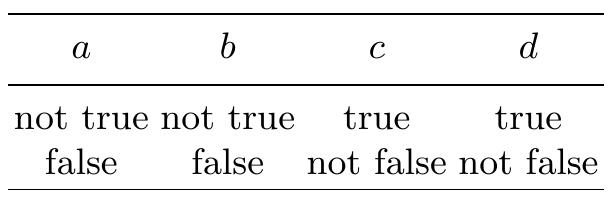
In constructing the three-valued logic, Jan Łukasiewicz was highly inspirited by the Aristotelian idea of logical contingency. Nevertheless, we can construct a four-valued logic for explicating the Stoic idea of logical determinacy. In this system, we have the following truth values: 0 ('possibly false), 1 ('necessarily false'), 2 ('possibly true'), 3 ('necessarily true'), where the designated truth value is represented by the two values: 2 and 3.